Module 4: Cost and Management Accounting — Notes
(Accounting for Managers – ACCT602, Semester I)
⚠️ Portal verification note: Module 4 is locked in the AMIGO course until Module 3 is marked complete, so this module's content is PDF-based only and has not yet been cross-checked against the live course (unlike Module 1, which is fully SCORM-verified). Ask me to continue the SCORM walkthrough if you want full portal verification here too.
4.1 Cost Sheet
Objectives of Cost Accounting
Determine selling price · Control cost (Budgetary Control, Standard Costing, Inventory Control) · Aid decision-making (make-or-buy, shut-down, replace machinery) · Ascertain costing profit · Help prepare financial statements faster.
Cost Classification (high-yield MCQ area)
flowchart TD
    A[Total Cost] --> B[Direct Material]
    A --> C[Direct Labour]
    A --> D[Direct Expenses]
    B & C & D --> E["Prime Cost = DM + DL + Direct Exp."]
    E --> F["+ Factory/Manufacturing Overheads"]
    F --> G["Works Cost / Factory Cost"]
    G --> H["+ Administration Overheads"]
    H --> I["Cost of Production"]
    I --> J["+ Selling & Distribution Overheads"]
    J --> K["Cost of Sales"]
    K --> L["+ Profit = Sales"]
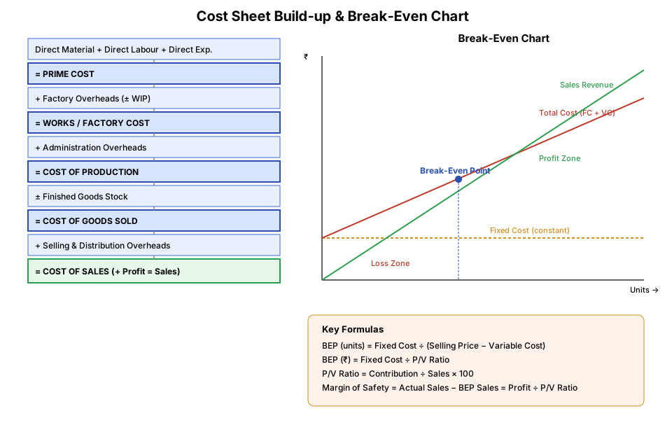
🧠 Memory trick — "Persistent Workers Carry Success": Prime Cost → Works/Factory Cost → Cost of Production → Cost of Sales (each step adds one more overhead layer: factory → admin → selling).
Key definitions: - Prime Cost = Direct Material + Direct Labour (+ Direct Expenses) - Conversion Cost = Direct Labour + Manufacturing Overhead - Product cost vs Period cost: product cost attaches to inventory (DM+DL+OH); period cost is expensed immediately (selling/admin costs). - Fixed vs Variable vs Semi-variable (mixed) cost — behaviour with activity level. - Direct vs Indirect cost — traceable to a cost object or not. - Decision-making costs: Differential cost (cost difference between alternatives), Opportunity cost (benefit foregone), Sunk cost (already incurred, irrelevant to future decisions).
Cost Sheet Format (memorise this — guaranteed numerical)
Opening Stock of Raw Material
+ Purchases (+ purchase expenses) − Closing Stock of RM
= Raw Material Consumed
+ Direct Wages + Direct Expenses
= PRIME COST
+ Factory Overheads (+ Opening WIP − Closing WIP)
= WORKS/FACTORY COST
+ Administration Overheads
= COST OF PRODUCTION
+ Opening Stock of Finished Goods − Closing Stock of Finished Goods
= COST OF GOODS SOLD
+ Selling & Distribution Overheads
= COST OF SALES
Profit (balancing figure) = Sales − Cost of Sales
4.2 Marginal Costing & CVP Analysis
Marginal Cost = cost of producing one additional unit (only variable costs).
Contribution & P/V Ratio
- Contribution = Sales − Variable Cost
- Net Profit = Contribution − Fixed Cost
- P/V Ratio = Contribution ÷ Sales × 100 (also = Change in Profit ÷ Change in Sales)
- Higher P/V ratio = more profitable product/better cost structure.
Break-Even Point (BEP) — very high-yield numerical
- BEP (units) = Fixed Cost ÷ (Selling Price per unit − Variable Cost per unit) = Fixed Cost ÷ Contribution per unit
- BEP (₹ sales) = Fixed Cost ÷ P/V Ratio
Margin of Safety (MOS)
- MOS = Actual Sales − Break-even Sales
- MOS = Profit ÷ P/V Ratio
- Improve MOS by: ↑ selling price, ↑ volume, better product mix, ↓ variable/fixed cost.
🧠 Memory trick — CVP chain: "Sales Vanish, Creating Fixed Profit" → Sales − Variable Cost = Contribution; Contribution − Fixed Cost = Profit. (BEP = the point where Contribution exactly equals Fixed Cost, so Profit = 0.)
flowchart LR
    Sales --> Contribution["Contribution = Sales − Variable Cost"]
    Contribution --> FC["Fixed Cost"]
    Contribution --> Profit["Profit = Contribution − Fixed Cost"]
    Contribution -->|"÷ Sales × 100"| PV["P/V Ratio"]
    FC -->|"÷ Contribution per unit"| BEP["Break-Even Point"]
    Profit -->|"÷ P/V Ratio"| MOS["Margin of Safety"]
4.3 Inventory Valuation
| Method | Logic | Effect (rising prices) |
|---|---|---|
| FIFO (First-In-First-Out) | Oldest stock issued/sold first | Closing stock at latest (higher) price → higher profit |
| LIFO (Last-In-First-Out) | Newest stock issued first | Closing stock at oldest (lower) price → lower profit (not allowed under Ind AS) |
| Weighted Average | Issue at weighted average cost | Smooths out price fluctuations |
Periodic system: stock counted physically at period-end. Perpetual system: running balance updated after every transaction.
🧠 Memory trick — FIFO vs LIFO: FIFO = "First In" gets sold First, so what's left (closing stock) is the newest, most expensive stock → higher profit when prices rise. LIFO = "Last In" gets sold First (Last-in, First-Out), so what's left is the oldest, cheapest stock → lower profit when prices rise (and LIFO isn't allowed under Ind AS).
4.4 Standard Costing & Variance Analysis
Standard Cost = predetermined cost used as a benchmark. Standard Costing = comparing actual vs standard to find variances → Management by Exception.
Material Variances (memorise these 3 formulas)
| Variance | Formula |
|---|---|
| Material Cost Variance (MCV) | (SP × SQ) − (AP × AQ) |
| Material Price Variance (MPV) | (SP − AP) × AQ |
| Material Usage/Quantity Variance (MUV) | (SQ − AQ) × SP |
Check: MCV = MPV + MUV — SP=Standard Price, SQ=Standard Qty, AP=Actual Price, AQ=Actual Qty
🧠 Memory trick for Price vs Usage/Efficiency variances — "PA-US": Price variance uses Actual quantity/hours held constant; Usage/efficiency variance uses Standard price/rate held constant. (Price variance = the OTHER factor is at Actual; Usage variance = the OTHER factor is at Standard.)
Labour Variances (mirror of material)
| Variance | Formula |
|---|---|
| Labour Cost Variance (LCV) | (SR × SH) − (AR × AH) |
| Labour Rate Variance (LRV) | (SR − AR) × AH |
| Labour Efficiency Variance (LEV) | (SH − AH) × SR |
SR=Standard Rate, SH=Standard Hours, AR=Actual Rate, AH=Actual Hours
flowchart TD
    MCV["Material Cost Variance\n(SP×SQ) − (AP×AQ)"] --> MPV["Price Variance\n(SP−AP)×AQ"]
    MCV --> MUV["Usage Variance\n(SQ−AQ)×SP"]
    LCV["Labour Cost Variance\n(SR×SH) − (AR×AH)"] --> LRV["Rate Variance\n(SR−AR)×AH"]
    LCV --> LEV["Efficiency Variance\n(SH−AH)×SR"]
4.5 Budgets
Budget = a quantitative/monetary plan for a future period. Budgeting = the process of preparing it. Budgetary Control = comparing actual vs budget and acting on variances.
Classification
| Basis | Types |
|---|---|
| Time | Long-term (5-10 yrs) · Short-term (1-2 yrs) · Current |
| Flexibility | Fixed Budget (one activity level) vs Flexible Budget (adjusts to actual activity level) |
| Function | Sales, Production, Cash, Purchase, Master Budget, etc. |
Fixed vs Flexible Budget — Exam favourite
| Basis | Fixed Budget | Flexible Budget |
|---|---|---|
| Activity level | Single | Multiple |
| Nature | Static | Dynamic |
| Comparison accuracy | Poor if activity differs | Good — adjusts to actual activity |
| Basis | Assumption | Realistic/practical |
Cash Budget: forecasts cash inflows/outflows over the budget period; ensures liquidity for operations — a common numerical topic (see 4.6.3 in Study Material).
Long-Answer Questions (15 Marks — model answers, ~300 words each)
Q1. Explain the elements of a Cost Sheet and how Prime Cost, Works Cost, Cost of Production, and Cost of Sales are derived. A Cost Sheet is a statement that presents the various components of the total cost of a product in a logical, layered format, building up from the most direct costs to the final selling price. It begins with Raw Material Consumed, computed as Opening Stock of Raw Material plus Purchases (and purchase-related expenses) minus Closing Stock of Raw Material. Adding Direct Wages and Direct Expenses (costs directly traceable to the specific product, like royalty on production or hire charges for special equipment) to Raw Material Consumed gives the Prime Cost — the most direct, traceable layer of cost. Next, Factory/Works Overheads — indirect manufacturing costs such as factory rent, power, depreciation on plant, and indirect labour — are added, along with adjustment for Opening and Closing Work-in-Progress (WIP), to arrive at the Works Cost (also called Factory Cost). Adding Administration Overheads — office rent, administrative salaries, and general management expenses not tied to production or selling — gives the Cost of Production. Adjusting this for Opening and Closing Stock of Finished Goods gives the Cost of Goods Sold. Finally, adding Selling and Distribution Overheads — advertising, sales commission, warehousing, and delivery costs — gives the Cost of Sales, and the difference between Sales revenue and Cost of Sales is the Profit (the balancing figure). This layered structure is valuable because it lets management see exactly where cost is being added at each stage of the product's journey from raw material to customer, supporting cost control, pricing decisions (ensuring selling price covers all cost layers plus desired margin), and comparison across periods or products to spot inefficiencies at a specific stage (e.g., rising works cost per unit might point to factory overhead creep rather than a raw-material price problem).
Q2. Explain Cost-Volume-Profit (CVP) Analysis. How are Break-Even Point and Margin of Safety calculated, and why are they important for managerial decisions? CVP Analysis studies the interrelationship between a company's costs, the volume of activity, and the resulting profit, helping management understand how changes in sales volume, price, or cost structure will affect profitability. Its foundation is splitting total cost into Fixed Cost (unchanged regardless of activity level, e.g., rent, salaries) and Variable Cost (changes proportionately with output, e.g., raw material, piece-rate wages). Contribution is Sales minus Variable Cost — it represents the amount available first to cover fixed costs, and then to generate profit; Profit itself equals Contribution minus Fixed Cost. The Profit-Volume (P/V) Ratio, calculated as Contribution ÷ Sales × 100, measures the profitability of the sales mix — a higher P/V ratio means a larger portion of every additional rupee of sales converts into profit. The Break-Even Point (BEP) is the sales level at which total contribution exactly equals fixed cost, so profit is zero — calculated in units as Fixed Cost ÷ Contribution per Unit, or in sales value as Fixed Cost ÷ P/V Ratio. Knowing BEP tells management the minimum sales volume needed just to avoid a loss, which is critical when launching a new product, evaluating a new market, or deciding on a major fixed-cost investment (like new machinery) that will raise the break-even threshold. The Margin of Safety (MOS) is the excess of actual (or budgeted) sales over the break-even sales — calculated as Actual Sales minus Break-even Sales, or equivalently as Profit ÷ P/V Ratio — and it measures the cushion a business has before it starts making losses; a low MOS signals high vulnerability to a sales downturn. Management can widen the margin of safety by raising selling prices, increasing sales volume, shifting the product mix toward higher-P/V-ratio products, or reducing variable/fixed costs. Together, BEP and MOS make CVP analysis indispensable for pricing decisions, sales targets, cost-structure planning (e.g., choosing between labour-intensive/low-fixed-cost versus automated/high-fixed-cost production), and assessing business risk.
Q3. Explain Standard Costing and Variance Analysis. Illustrate Material Cost Variance and its sub-variances. Standard Costing is a technique in which predetermined ("standard") costs — for material, labour, and overheads — are set in advance based on efficient operating conditions, and actual costs incurred are then compared against these standards to compute variances. This comparison embodies the principle of Management by Exception — rather than scrutinising every transaction, management's attention is drawn only to significant deviations from standard, allowing efficient, focused control. For direct material, the key variance is the Material Cost Variance (MCV), calculated as (Standard Price × Standard Quantity) − (Actual Price × Actual Quantity) — it captures the total difference between what the output should have cost in materials and what it actually cost. This total variance is then decomposed into two more diagnostic sub-variances. The Material Price Variance (MPV), calculated as (Standard Price − Actual Price) × Actual Quantity, isolates how much of the total variance is due purely to paying more or less than the standard price per unit of material — this might result from supplier price changes, bulk-discount negotiation, or a change in vendor, and is typically the responsibility of the purchasing department. The Material Usage/Quantity Variance (MUV), calculated as (Standard Quantity − Actual Quantity) × Standard Price, isolates how much of the variance is due to using more or less material than the standard allows for the actual output — this might result from wastage, pilferage, or a change in production efficiency, and is typically the responsibility of the production department. Together, MCV = MPV + MUV always holds, and this decomposition is powerful because it pinpoints which department should be held accountable: an adverse total variance caused entirely by a price variance shouldn't be blamed on the shop floor, and vice versa. The same logic mirrors for labour, giving Labour Cost Variance, Labour Rate Variance, and Labour Efficiency Variance, making variance analysis a core tool for cost control and departmental performance evaluation.
Q4. Differentiate between Fixed Budget and Flexible Budget, and explain the importance of budgetary control. A Budget is a quantitative and/or monetary plan for a future period, and Budgetary Control is the ongoing process of comparing actual performance against the budget, analysing variances, and taking corrective action — essentially planning combined with continuous control. Budgets are classified along several dimensions, but the most commonly tested distinction is between Fixed and Flexible budgets. A Fixed Budget is prepared for a single, predetermined level of activity and does not change even if actual activity differs — it works well only in stable, predictable environments, but becomes a poor and even misleading benchmark when actual output diverges significantly from the assumed level, since costs that vary with volume (like raw material) would naturally differ from the fixed budget even if the business performed perfectly efficiently at its actual volume. A Flexible Budget, in contrast, is designed to adjust automatically to the actual level of activity achieved — it separates costs into fixed and variable components in advance, so that at any given activity level, a corresponding budget figure can be recalculated and compared fairly against actual results. This makes flexible budgeting far more realistic and useful for performance evaluation, because it isolates genuine efficiency variances (did we spend more/less than we should have at the volume we actually achieved?) from simple volume effects (we spent more only because we produced more). Budgetary control matters for several reasons: it forces forward planning and coordination across departments (sales, production, purchase, and cash budgets must all be mutually consistent, typically consolidated into a Master Budget); it establishes performance benchmarks against which actual results and individual managers can be evaluated; it highlights problem areas early through variance analysis, enabling timely corrective action; and a Cash Budget specifically ensures the business maintains adequate liquidity by forecasting cash inflows and outflows, preventing the common scenario where a profitable business still runs into a cash crunch from poor short-term cash planning.
Live course walkthrough (verified against the AMIGO SCORM module, 28 lessons)
The sections above were built from the PDF. Everything from here on is taken from the live course, lesson by lesson, and the live course wins wherever the two differ.
Lesson 1: Learning Objectives
Define cost and management accounting; explain the cost sheet with an example; describe marginal costing; analyse CVP analysis and the margin of safety; apply CVP to decision making; explain inventory valuation basics and compare methods; analyse material and labour variances; describe budgeting fundamentals, budget types and advanced budget types.
Lesson 2: Introduction
- Cost accounting arose because financial accounting (gross profit, P&L, balance sheet) does not give the detailed cost data management needs for planning, decision making and control.
- Cost accounting = classification, accumulation, control and assignment of costs; it produces internal reports giving cost per unit of articles or jobs and cost at various stages of completion. It is directly concerned with inventory control, plant asset management and allocation of funds to functional activities.
- Management accounting is a more recent branch: it supplies information for policy development, planning, organisation, staffing, direction and control.
Lesson 3: 4.1.1 Cost & Management Accounting - Introduction (7 min, SLM p.143-144)
- Cost accounting documents, classifies, distributes and records current and potential costs, to ascertain the cost of products or services and to show avoidable losses and waste. Management accounting gives management relevant information to take control decisions at the right time.
- Objectives of cost accounting (5 accordions): 1. Determining the selling price (cost is a key factor alongside quality, market conditions, distribution area and quantity). 2. Controlling cost (budgetary control, standard costing, inventory control; actuals compared with budgets). 3. Decision making (cost-volume-profit relationship; make or buy; shut down or continue at a loss; replace machinery). 4. Ascertaining costing profit or loss on an objective basis by matching cost with revenue. 5. Facilitating preparation of financial statements at short intervals (daily/weekly/monthly statements, immediate stock information).
- Quizzes: see Quiz Bank Q1-2.
Lesson 4: 4.1.2 Cost Classification (22 min, SLM p.144-148)
- Cost is the money spent to produce a product or provide a service. Different uses need different classifications: external reports use historical cost; decisions use predicted future costs.
- Manufacturing costs: direct material, direct labour, manufacturing overhead.
- Direct material = opening stock + purchases - closing stock (e.g. wood for furniture, cotton for yarn).
- Direct labour ("touch labour") is traceable to units (assembly workers, carpenters, machine operators); supervisors, material handlers and night guards are indirect labour.
- Prime cost = direct materials + direct labour (e.g. 4,500 + 3,000 = 7,500).
- Manufacturing overhead = all other manufacturing costs (indirect material and labour, repairs, heat and light, depreciation and insurance on factory), also called factory overhead or factory burden.
- Conversion cost = direct labour + manufacturing overhead (e.g. 3,000 + 2,000 = 5,000).
- Non-manufacturing costs: marketing or selling costs (order getting and order filling: advertising, shipping, sales commission, sales salaries) and administrative costs (executive pay, general accounting, secretarial, public relations).
- Product cost vs period cost (flashcards): product costs = direct materials, direct labour and manufacturing overhead for manufactured goods; period costs = everything not in product cost, so all non-manufacturing costs.
- Cost behaviour (accordions): variable cost varies in total in direct proportion to activity (direct material); fixed cost stays constant in total regardless of activity (rent, straight-line depreciation, supervisory salary), though per-unit fixed cost falls as activity rises; mixed (semi-variable) cost has both elements, y = a + bX.
- Direct vs indirect cost (tabs): a direct cost is easily traceable to a cost object (a regional sales manager's salary for that office); an indirect cost is not (a factory manager's salary in a soup factory making several varieties); a common cost supports several cost objects and is a type of indirect cost.
- Decision-making costs (accordions): differential cost (difference in cost between alternatives; incremental or decremental); quality costs (prevention, appraisal, internal failure, external failure); opportunity cost (benefit foregone, e.g. Rs 400 weekly wage lost by taking a week at the beach); sunk cost (already incurred, unrecoverable, ignored in decisions, e.g. Rs 60,000 obsolete machine).
- Quizzes: see Quiz Bank Q3-4.
Lesson 5: 4.1.3 Cost Sheet Part 1 - Explaining the Sheet (6 min, SLM p.148-149)
- A cost sheet is a statement of cost: costing information set out as a statement. Used when one product is made and all costs are for that product. It can be prepared weekly, monthly, quarterly or yearly and shows prime cost, works cost, cost of production, cost of goods sold, total cost and profit.
- Three types (tabs): 1. Cost sheet with break-up cost: two columns, total cost and cost per unit of output. 2. Cost sheet with treatment of stock: for manufacturing concerns; stocks of raw material, work in progress and finished goods are handled in a separate proforma. 3. Estimated cost sheet or price quotation: quotation means quoting the minimum price to win a specific order; one column; estimated direct material, estimated labour cost and estimated overheads.
- Quizzes: Quiz Bank Q5-6 (prime cost is the largest component of total cost; "acts as an agent to manufacturer" is not an advantage of a cost sheet).
Lesson 6: 4.1.4 Cost Sheet Part 2 - Numerical Example (10 min, SLM p.149-151)
- Worked example for "Centre Corporation" (1-30 January 2010): the transactions table and the solved cost sheet are images in the course. The solved sheet runs through prime cost, factory/works cost, cost of production, cost of goods sold, cost of sales and profit.
- Standard cost-sheet build-up: Prime cost = direct material + direct labour + direct expenses; add factory overheads for works cost; add administration overheads for cost of production; adjust opening/closing finished stock for cost of goods sold; add selling and distribution overheads for cost of sales; add profit for sales.
- Quizzes: Quiz Bank Q7-8 (production cost = 40,000 + 25,000 + 15,000 = 80,000; cost per unit = 150,000 / 600 = 250).
Lesson 7: 4.2.1 Marginal Costing - Meaning and Purpose (5 min, SLM p.152)
- Marginal cost is the change in total cost when output changes by one unit, i.e. the cost of producing one more unit. ICMA London: the amount at any volume of output by which aggregate costs change if output is increased or decreased by one unit.
- It includes all costs that vary with the production level. The purpose of marginal cost analysis is to find the point at which economies of scale are reached so output and operations are maximised. When the marginal cost of one extra unit is below the price per unit, the manufacturer can make a profit.
- Uses: make-or-buy decisions (buy only if the supplier's price is below marginal cost), key-factor (limiting factor) decisions, closure of a department, product mix.
- Quizzes: Quiz Bank Q9-10.
Lesson 8: 4.2.2 CVP Analysis - Contribution, P/V Ratio (13 min, SLM p.152-154)
- CVP analysis examines the relationships between costs, volume and profit. It rests on five elements (flashcards): price of products, volume or level of activity, per-unit variable cost, total fixed cost, and mix of products sold. It guides what to make or sell, pricing policy, marketing strategy and which facilities to acquire.
- Contribution margin = sales revenue - variable cost. It covers fixed expenses first and then profit; if it is too small to cover fixed cost, there is a loss. Contribution - fixed cost = net operating income or loss.
- P/V (profit-volume) ratio = contribution / sales (also called marginal income ratio, contribution-to-sales ratio, variable profit ratio) = (sales - variable cost) / sales = 1 - variable cost / sales = (fixed cost + profit) / sales = change in profit (or contribution) / change in sales. It is the rate at which profit grows with volume.
- A higher P/V ratio means higher profitability. Improve it by raising the selling price, cutting direct and variable costs, or switching to products with a higher P/V ratio.
- Profit at any sales volume: Volume x P/V ratio = Contribution; Contribution - fixed costs = Profit.
- Limitations of CVP: assumes capacity and the elements of cost remain the same; forecasting profit is hard when many products are sold.
- Quizzes: Quiz Bank Q11-12.
Lesson 9: 4.2.3 CVP Analysis - Break-Even Analysis (4 min, SLM p.154-156)
- Break-even analysis studies the relationship between total sales, total expenses and total income at different production rates, to find the revenue needed to break even and the gain or loss at every sales point.
- BEP (units) = Fixed costs / (Selling price per unit - Variable cost per unit). BEP in sales rupees = BEP units x selling price (worked example: 350 units x Rs 250 = Rs 87,500). A second example gives BEP of 20,000 units and Rs 1,60,000 of sales.
- Assumptions: all costs are perfectly variable or absolutely fixed over the period; production equals sales volume; revenue varies perfectly with physical volume; product mix is stable. In reality demand swings, inventory, pricing and mix changes break these.
- Advantages (10): shows the output level below which production is not profitable; target capacity for minimum unit cost; minimum cost for a given output; make-or-buy decisions; plant expansion or contraction; price-change and profit analysis; dropping or adding a product; percentage yield of a project and choice among projects; most profitable selling price; the point from which dividends can start to be paid.
- Quizzes: Quiz Bank Q13-14 (10,000 / (10 - 6) = 2,500 units; with desired profit, (10,000 + 9,000) / 4 = 4,750 units).
Lesson 10: 4.2.4 CVP Analysis - Margin of Safety (20 min, SLM p.156-157)
- Margin of safety (MoS) = actual sales - break-even sales = profit / P/V ratio. It is how far sales can fall before losses begin; larger MoS means lower risk. It is advisable to keep a margin of safety of at least 50% to meet long-term obligations; below that the firm risks defaulting on interest.
- MoS as a % of sales = (actual sales - BEP sales) / actual sales x 100.
- Ways to improve MoS (flashcards): raise the selling price; increase production; change the product mix; reduce variable cost; reduce fixed cost.
- Quizzes: Quiz Bank Q15-16 (the course's Firm A data sit in images; the keys were 70 and 57.14).
Lesson 11: 4.2.5 CVP Analysis - Decision Making, Examples (20 min, SLM p.157-160)
- Break-even analysis uses cost data to make decisions; two key methods (flashcards): break-even charts and the algebraic method.
- Profit contribution = price - average variable cost (P - AVC). At low sales the contribution has not yet covered fixed cost, so there is a loss; once fixed costs are covered, the firm makes a profit.
- Break-even chart: a graph of output/sales against revenue and cost. Total revenue (TR) is a straight line (constant price); total cost (TC) starts at the vertical intercept TFC and rises with slope = constant AVC. The break-even point is where TR = TC (output Q1); below it the firm makes a loss, above it a profit. Both lines are linear because price and variable cost per unit are assumed constant.
- Algebraic method: TR = P x Q; TC = TFC + AVC x Q; set TR = TC and solve for the break-even output QB = TFC / (P - AVC). To earn a desired profit R: Q = (TFC + R) / (P - AVC).
- Worked example (Quick Standards Ltd): contribution, then P/V ratio, then break-even sales = fixed cost / P/V ratio, margin of safety two ways (actual sales - BEP sales, or profit / P/V ratio), and sales needed for a Rs 6,000 profit = (fixed cost + profit) / P/V ratio. The numbers are in images.
- Assumptions of CVP: revenues change proportionately with volume; constant product mix; the analysis is deterministic; volume alone drives changes in costs and revenues.
- Quizzes: Quiz Bank Q17-18.
Lesson 12: 4.3.1 Inventory Valuation - Introduction, Periodic, Perpetual and FIFO (12 min, SLM p.160-162)
- Inventory (stock) = assets held for sale, in the process of production for sale, or to be used in producing goods.
- Periodic inventory valuation (tab): stock is physically counted at defined intervals (e.g. period end) and the count balances the general ledger. Advantages: no counting between periods (smaller workforce), quantity is physically verified, regular work is not interrupted. Weakness: minimal information between periods, so large adjustments may be needed at the end.
- Perpetual inventory valuation (tab): stock records are updated continuously with every receipt and issue.
- The costing method chosen affects the balance sheet, income statement and cash flow statement. Three widely used methods: FIFO, LIFO and average cost.
- FIFO (first in, first out): the first units received are assumed to be the first sold. Bakery example: 200 loaves at Rs 1 on Monday and 200 at Rs 1.25 on Tuesday; selling 200 on Wednesday gives COGS of Rs 1 per loaf, and the Rs 1.25 loaves stay in ending inventory.
- Illustration 1 (stores ledger by FIFO, opening balance 200 units at Rs 25): closing stock on 31 Dec 2014 = 50 units at Rs 23.50 = Rs 1,175.
- FIFO disadvantages: two similar jobs cannot be compared because different material rates are used; when prices fall, material cost charged to production is high, giving high quotations; when prices rise, the earliest (cheapest) materials are issued first, which lowers COGS and raises gross profit. Closing stock does reflect current market price (an advantage).
- Quizzes: Quiz Bank Q19-20.
Lesson 13: 4.3.2 Inventory Valuation - LIFO & Average Methods (SLM p.162-165)
- LIFO: assumes the last unit into inventory is sold first, so older stock remains at period end (bakery example: the 200 loaves sold on Wednesday are costed at Rs 1.25, the remaining Rs 1 loaves value closing inventory). Worked ledger examples: Poplive Co. and Krishna & Sons.
- Average cost: each unit is costed at the weighted average of units available (bakery average Rs 1.125); specific identification tracks each item's own cost. Average method simplifies calculation and record keeping, suits goods that cannot be told apart (oil, wheat, iron ore) and is permitted by accounting standards such as IFRS; LIFO is not permitted under IFRS.
- Quizzes (both answers missed; platform keys: LIFO prices issues at the most recent lots; the "not permitted under IFRSs" statement was keyed for the average-method question - flagged as unreliable). Not added to the Quiz Bank as verified.
Lesson 14: 4.4.1 Standard Costing & Variance Analysis - Introduction (SLM p.166-167)
- Standard cost: predetermined cost used as a yardstick to judge efficiency of actual costs (e.g. the quantity of raw material per unit and its estimated price give the standard material input). Standard costing compares actual production results with the standard cost model to find reasons for differences.
- Salient features: set standard costs for each cost element (materials, labour, expenses); compare actual with standard to identify variances; record standards and actuals simultaneously; identify causes; report variances to management.
- Objectives (6 markers): (1) cost control (yardstick against which actual costs are compared, corrective action); (2) management by exception (attention only where performance deviates); (3) cost-conscious attitude; (4) price fixation (quotations, tenders); (5) fixing prices and formulating policies (profit planning, product and inventory pricing); (6) management planning (budgets are easier on standards).
- Variance: difference between actual and standard; favourable if actual cost is lower (or result better), unfavourable/adverse if higher. Principles: state variances in money; analyse product-wise; favourable or adverse; total cost variance = standard cost of actual output minus actual cost.
- Quizzes: Quiz Bank Q21-22.
Lesson 15: 4.4.2 Variance Analysis: Material (SLM p.167-169)
- Material variances: cost, price, usage (quantity), mix (4 tabs).
- Material cost variance MCV = (SP x SQ) - (AP x AQ) (SP standard price, SQ standard quantity, AP actual price, AQ actual quantity).
- Price variance: due to difference between standard and actual price per unit, on the total quantity purchased (reasons: prices higher or lower than planned, discounts, quality, substitutes). Usage variance: difference in quantity used vs standard (reasons: yield, substitutes, scrap, quality differences). Mix variance: arises when the ratio of materials deviates from the standard mix; Material Mix Variance = Standard rate x (Standard quantity - Actual quantity).
- Quizzes: Quiz Bank Q23-24.
Lesson 16: 4.4.3 Variance Analysis: Labour (SLM p.169-171)
- Labour variances mirror material variances (4 tabs): cost LCV = (SR x SH) - (AR x AH); rate LRV = (SR - AR) x AH (wage-rate difference); efficiency (actual vs standard hours at the standard rate); mix LMV = SR x (Revised standard time - Actual time). A lower actual labour cost than standard is favourable, higher is adverse. A worked example (grade A and B workers, standard Rs 100 per unit, 80 units made) computes the labour mix variance.
- Quizzes: Quiz Bank Q25-26 (rate-variance reasons: key says "payment of no bonus" is the item that is not a reason; efficiency-variance item not a reason: "good supervision").
Lesson 17: 4.5.1 Budget and Budgeting: Introduction and Types of Budgets (SLM p.171-172)
- Budget: a plan and blueprint for planned action, in monetary terms, prepared before the period to attain an objective. Objectives of budget (5 markers): focus everyone on a shared objective; coordinate departments; meticulous control over each function's performance and cost; built bottom-up and managed top-down; compare budgets against actual performance.
- Budgeting = the process of formulating budgets (analysing business conditions, management priorities and capacity). Objectives of budgeting: more economical use of capital; coordination of functions; plan and control income and expenditure; good business practice by planning ahead; match sales with production; assign departmental responsibilities; prevent wastage; ensure working capital availability.
- Budgeting process (carousel): (1) objective determination: broad, long-range, qualitative; (2) goal determination: specific quantitative targets; (3) strategy formulation: methods or courses of action to achieve goals.
- Quizzes: Quiz Bank Q27-28.
Lesson 18: 4.5.2 Types of Budgets - Part 1
- Budgets are classified by operational features of the business: on the basis of time and on the basis of functions.
- On the basis of time: Long-term budgets (5 to 10 years; business forecasting and future planning); Short-term budgets (one or two years; often a production plan in monetary terms); Current budgets (related to present conditions, short-term use, more practical than basic budgets because targets are adjusted to current conditions).
- A budget is a quantitative plan that estimates future operations. Fixed budget: stays constant irrespective of activity level (created for a standard volume of production). Flexible budget: created for different production levels or capacity utilisation; it changes with the activity level.
- Quiz: a statement of planned sales in quantity and value, analysed by products = sales budget. A budget for procuring goods to meet the sales target and inventory = purchase budget (my pick was marked incorrect by the platform; key not revealed, so not added to the Quiz Bank as verified).
Lesson 19: 4.5.3 Types of Budgets - Part 2
- On the basis of functions: (a) functional budgets and (b) the master budget.
- Functional budgets: (1) Sales budget - forecast of total sales in money and quantity; quantity first, then converted to money; usually the first step because sales are the primary budget factor; classified by products, areas, salesmen/agents, customer types and periods. (2) Production budget - prepared by the production manager, in units, based on the sales budget; has a volume part and a cost part; considers plant utilisation, raw material and labour; avoids overwork in busy periods and keeps minimum finished-goods stock. (3) Purchase budget - purchases of direct and indirect materials and services (and finished goods for resale), in quantity or money; based on sales and production budgets, capital expenditure budget, R&D cost budget and orders already placed. (4) Administration cost budget - estimated cost of formulating policy, directing and controlling; mostly fixed so easiest to prepare. (5) Capital expenditure budget - estimated spending on fixed assets (new plant, replacement, improved machinery).
- Cash budget: shows flow of funds and needs - cash from cash and credit sales, payments to suppliers and other capital and revenue expenses; shows when overdrafts or loans must be arranged.
- Master budget: prepared from and summarises the functional budgets (also called summary budget): budgeted profit and loss account and budgeted balance sheet (possibly a budgeted cash flow statement). Prepared by the budget committee; once approved it is the enterprise's target for the period; like financial statements but on expected future data.
Lesson 20: 4.6.1 Numerical - CVP Analysis
- Worked example: Sales Rs 1,00,000, total cost Rs 75,000, fixed cost Rs 20,000, net profit Rs 25,000. Variable cost = 75,000 - 20,000 = 55,000; contribution = 45,000. P/V ratio = contribution / sales = 45%. Break-even point = fixed cost / P/V ratio = 20,000 / 0.45 = about Rs 44,444. Margin of safety = profit / P/V ratio = 25,000 / 0.45 = about Rs 55,556 (or actual sales - BEP sales).
- Quiz (alarm clocks: variable cost Rs 40, fixed cost Rs 60,000, selling price Rs 60): contribution per unit = Rs 20, so BEP = 60,000 / 20 = 3,000 clocks; units for a profit of Rs 40,000 = (60,000 + 40,000) / 20 = 5,000 clocks. Both verified correct on the platform.
Lesson 21: 4.6.2 Numerical - Variance Analysis (long lesson, many worked examples)
- Material variances example: standard 10 kg per unit at Rs 25/kg; actual 11,500 kg costing Rs 2,75,000 for 1,000 units. Standard cost = 10,000 kg x 25 = 2,50,000. Material cost variance = SC - AC = 2,50,000 - 2,75,000 = 25,000 (A). Material price variance = (SP - AP) x AQ = 2,87,500 - 2,75,000 = 12,500 (F). Material usage variance = (SQ - AQ) x SP = (10,000 - 11,500) x 25 = 37,500 (A). Check: MCV = MPV + MUV.
- Further worked examples: material price variance (std 25 units at Rs 5; actual 20 units at Rs 4), material mix variance (sum of usage variances per ingredient at standard rates), labour mix variance (Grade A and B workers), plus CVP examples (P/V ratio before and after a 10% price cut, break-even sales, profit at +5% / -10% sales, shirt retailer with salaries, office costs, advertising, commission and 15% price rise).
- Quiz (standard output 100 units, 3 kg per unit, std price Rs 2; actual output 80 units, actual price Rs 2.50, 250 kg used): my picks "125 (A) and 20 (A)" for price and usage variance and "145 (A)" for cost variance were marked incorrect and no key was revealed, so they are not recorded as verified. (Textbook method on actual output gives MPV 125 A, MUV 20 A, MCV 145 A; the platform key probably uses the standard output of 100 units: MUV 100 F, MCV 25 A.)
Lesson 22: 4.6.3 Numerical - Budgets (Cash Budget)
- Exercise: prepare a cash budget for January-April with opening bank balance Rs 8,000 and Rs 5,000 monthly earnings; financing rule: bank arrangement if the deficit is under Rs 10,000, debentures if the deficit is above Rs 10,000 and under Rs 42,000, share issue if the deficit is above Rs 42,000 (within authorised capital).
- Quiz: wages forecast Dec 4,800, Jan 6,000, Feb 6,400, Mar 6,800 with a 1/8 month payment lag: wages paid = 7/8 of the current month + 1/8 of the previous month = Rs 5,850 (Jan), Rs 6,350 (Feb), Rs 6,750 (Mar) (verified correct). The credit-sales question ("sales amount for February with 2 months credit, January + February sales Rs 9,000") was answered "Insufficient information" and marked incorrect; key not revealed.
Lesson 23: Summary
- Cost accounting deals with documentation, classification, distribution and recording of current and potential costs; aim: ascertain the cost of products or services and show avoidable losses and waste.
- Cost sheet: a statement of cost; usually adopted when only one product is produced and all costs relate to it.
- Marginal cost: all costs that vary with the production level; the sum varies with the volume produced.
- Break-even analysis: relationship between total sales, total expenses and total income at different production rates; shows the revenue needed to break even and gains or losses at each sales point.
- Margin of safety: actual sales minus break-even sales; the amount by which sales can fall before losses begin.
- LIFO: the last unit into inventory is sold first; older inventory is left at period end (bakery example: 200 loaves sold on Wednesday at Rs 1.25 go to COGS, the remaining Rs 1 loaves value closing inventory).
- Standard costs: predetermined costs used as a yardstick to measure efficiency (e.g. standard material input per unit).
- Standard costing objectives: classification and computation of variances for direct material, direct labour and overheads.
- Cash budget: shows flow of funds and needs - cash and credit sales receipts and cash payments (capital and revenue).
Lesson 24: Glossary
- Marginal cost: cost of producing additional units, including all costs that vary with production level.
- Margin of safety: difference between actual sales and break-even point; how far sales can drop before losses.
- Inventory: assets intended for sale, in the process of being produced for sale, or to be used in producing goods.
- LIFO: inventory valuation assuming the last units purchased or produced are sold first.
- Standard costing: uses standard costs for direct materials, direct labour and overhead to compare with actual costs and identify variances.
Lesson 25: Check Your Understanding
- 5-question quiz (pass mark 0%); scored 100%. Questions in Quiz Bank Q35-39.
Lesson 26: Exercise (notebook)
- How are costs classified in cost accounting? 2. What is marginal costing and how does it differ from absorption costing? 3. Explain break-even analysis and its importance in decision making. 4. How is the margin of safety calculated in CVP analysis? 5. How does inventory valuation impact a company's financial statements?
Lesson 27: Learning Activities
- Given a list of costs (direct material, direct labour, manufacturing overhead, selling and administrative expenses), classify each as variable or fixed and as product or period cost. 2. Prepare a cost sheet for a given product showing direct material, direct labour, manufacturing overhead and total cost per unit.
Lesson 28: Further Readings and Bibliography
- Horngren, Accounting for Management Control (Prentice Hall, 1965); Maheswari, Management Accounting (Sultan Chand); Hingorani, Ramanathan and Grewal, Management Accounting; Jain and Narang, Cost Accounting.
✨ Quick Revision Pack (Module 4)
60-second summary
- Cost accounting records and analyses costs; management accounting uses information for decisions. Cost sheet builds up: Prime cost → Factory cost → Cost of production → Cost of goods sold → Total cost → Sales price (with profit).
- Marginal costing: only variable costs go into product cost; fixed costs are period costs. Contribution = Sales - Variable cost.
- CVP: P/V ratio = Contribution / Sales; BEP (units) = Fixed cost / Contribution per unit; BEP (value) = Fixed cost / P/V ratio; Margin of safety = Actual sales - BEP sales = Profit / P/V ratio.
- Inventory valuation: FIFO, LIFO, weighted average; periodic vs perpetual.
- Standard costing: variance = standard cost - actual cost (Favourable / Adverse); material, labour, overhead variances.
- Budgets: sales, production, purchase, cash, master, fixed vs flexible; cash budget shows funds flow.
Diagrams
Cost sheet build-up
flowchart TB
  A["Direct material + Direct labour + Direct expenses = PRIME COST"] --> B["+ Factory overheads = FACTORY COST"] --> C["+ Opening WIP - Closing WIP = COST OF PRODUCTION"] --> D["+ Administration overhead (+ opening, - closing finished goods) = COST OF GOODS SOLD"] --> E["+ Selling and distribution overhead = TOTAL COST"] --> F["+ Profit = SALES"]
Break-even logic
flowchart LR
  S["Sales"] --> C["- Variable cost = Contribution"] --> F["- Fixed cost"] --> P["= Profit or loss"]
  C --> B["Break-even when Contribution = Fixed cost"]
Variance tree (material)
flowchart TB
  MCV["Material cost variance = SC - AC"] --> MPV["Price variance = (SP - AP) x AQ"]
  MCV --> MUV["Usage variance = (SQ - AQ) x SP"]
Memory tricks
BEP = Fixed ÷ Contribution ("fixed costs recovered by contribution"). Units: divide by contribution per unit; value: divide by P/V ratio.
Variance sign: Favourable when actual is better than standard (lower cost, higher income). Price variance uses actual quantity; usage variance uses standard price.
Margin of safety = Profit ÷ P/V ratio. It is the cushion by which sales can fall before losses start.
FIFO vs LIFO (rising prices): FIFO → higher closing stock, higher profit; LIFO → higher COGS, lower profit and tax.
In marginal costing, fixed costs are not carried into inventory – so profit can differ from absorption costing when stock levels change.
Formula sheet
| Concept | Formula |
|---|---|
| Contribution | Sales - Variable cost |
| P/V ratio | Contribution / Sales x 100 |
| BEP units | Fixed cost / (Selling price - Variable cost per unit) |
| BEP sales | Fixed cost / P/V ratio |
| Sales for target profit | (Fixed cost + Target profit) / P/V ratio |
| Margin of safety | Actual sales - BEP sales |
| Material usage variance | (SQ - AQ) x SP |
| Material price variance | (SP - AP) x AQ |
| Labour rate variance | (SR - AR) x actual hours |
| Labour efficiency variance | (SH - AH) x SR |
Practice problems (with answers)
- P/V and BEP: sales 1,00,000; variable cost 55,000; fixed cost 20,000. → Contribution 45,000; P/V = 45%; BEP = 20,000/0.45 = Rs 44,444; profit = 25,000; margin of safety = 25,000/0.45 = Rs 55,556.
- Alarm clocks: price Rs 60; variable Rs 40; fixed Rs 60,000. → Contribution 20; BEP = 3,000 units; for Rs 40,000 profit = (60,000 + 40,000)/20 = 5,000 units.
- Material variances: standard 10 kg x Rs 25 = Rs 250 per unit, 1,000 units; actual 11,500 kg costing Rs 2,75,000. → MCV = 2,50,000 - 2,75,000 = 25,000 A; MPV = (25 - 23.91) x 11,500 = 12,500 F; MUV = (10,000 - 11,500) x 25 = 37,500 A (12,500 F - 37,500 A = 25,000 A).
- Cost sheet: DM 40,000; DL 20,000; direct exp 5,000; factory OH 15,000; admin OH 10,000; selling OH 8,000; profit 20%. → Prime cost 65,000; factory cost = cost of production 80,000; cost of goods sold (add admin 10,000) 90,000; total cost (add selling 8,000) 98,000; sales at 20% on cost = Rs 1,17,600 (or 20% on sales = 1,22,500).
- Cash budget: wages Dec 4,800; Jan 6,000 with 1/8 paid next month. → Jan payment = 7/8 x 6,000 + 1/8 x 4,800 = Rs 5,850.
- Short answer (5 marks): Why use marginal costing for decisions? → It separates variable and fixed costs, shows contribution per product, supports make-or-buy, pricing, product-mix and shutdown decisions, and is not distorted by fixed cost allocation.