Module 4: Introduction to Cost and Management Accounting
(Accounting for Managers – ACCT602, Semester I)
⚠️ Portal verification note: Module 4 is locked in the AMIGO course until Module 3 is marked complete, so this module's content is PDF-based only and has not yet been cross-checked against the live course (unlike Module 1, which is fully SCORM-verified). Ask me to continue the SCORM walkthrough if you want full portal verification here too.
4.1 Cost Sheet
Objectives of Cost Accounting
Determine selling price · Control cost (Budgetary Control, Standard Costing, Inventory Control) · Aid decision-making (make-or-buy, shut-down, replace machinery) · Ascertain costing profit · Help prepare financial statements faster.
Cost Classification (high-yield MCQ area)
flowchart TD
    A[Total Cost] --> B[Direct Material]
    A --> C[Direct Labour]
    A --> D[Direct Expenses]
    B & C & D --> E["Prime Cost = DM + DL + Direct Exp."]
    E --> F["+ Factory/Manufacturing Overheads"]
    F --> G["Works Cost / Factory Cost"]
    G --> H["+ Administration Overheads"]
    H --> I["Cost of Production"]
    I --> J["+ Selling & Distribution Overheads"]
    J --> K["Cost of Sales"]
    K --> L["+ Profit = Sales"]
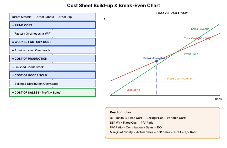
🧠 Memory trick — "Persistent Workers Carry Success": Prime Cost → Works/Factory Cost → Cost of Production → Cost of Sales (each step adds one more overhead layer: factory → admin → selling).
Key definitions: - Prime Cost = Direct Material + Direct Labour (+ Direct Expenses) - Conversion Cost = Direct Labour + Manufacturing Overhead - Product cost vs Period cost: product cost attaches to inventory (DM+DL+OH); period cost is expensed immediately (selling/admin costs). - Fixed vs Variable vs Semi-variable (mixed) cost — behaviour with activity level. - Direct vs Indirect cost — traceable to a cost object or not. - Decision-making costs: Differential cost (cost difference between alternatives), Opportunity cost (benefit foregone), Sunk cost (already incurred, irrelevant to future decisions).
Cost Sheet Format (memorise this — guaranteed numerical)
Opening Stock of Raw Material
+ Purchases (+ purchase expenses) − Closing Stock of RM
= Raw Material Consumed
+ Direct Wages + Direct Expenses
= PRIME COST
+ Factory Overheads (+ Opening WIP − Closing WIP)
= WORKS/FACTORY COST
+ Administration Overheads
= COST OF PRODUCTION
+ Opening Stock of Finished Goods − Closing Stock of Finished Goods
= COST OF GOODS SOLD
+ Selling & Distribution Overheads
= COST OF SALES
Profit (balancing figure) = Sales − Cost of Sales
4.2 Marginal Costing & CVP Analysis
Marginal Cost = cost of producing one additional unit (only variable costs).
Contribution & P/V Ratio
- Contribution = Sales − Variable Cost
- Net Profit = Contribution − Fixed Cost
- P/V Ratio = Contribution ÷ Sales × 100 (also = Change in Profit ÷ Change in Sales)
- Higher P/V ratio = more profitable product/better cost structure.
Break-Even Point (BEP) — very high-yield numerical
- BEP (units) = Fixed Cost ÷ (Selling Price per unit − Variable Cost per unit) = Fixed Cost ÷ Contribution per unit
- BEP (₹ sales) = Fixed Cost ÷ P/V Ratio
Margin of Safety (MOS)
- MOS = Actual Sales − Break-even Sales
- MOS = Profit ÷ P/V Ratio
- Improve MOS by: ↑ selling price, ↑ volume, better product mix, ↓ variable/fixed cost.
🧠 Memory trick — CVP chain: "Sales Vanish, Creating Fixed Profit" → Sales − Variable Cost = Contribution; Contribution − Fixed Cost = Profit. (BEP = the point where Contribution exactly equals Fixed Cost, so Profit = 0.)
flowchart LR
    Sales --> Contribution["Contribution = Sales − Variable Cost"]
    Contribution --> FC["Fixed Cost"]
    Contribution --> Profit["Profit = Contribution − Fixed Cost"]
    Contribution -->|"÷ Sales × 100"| PV["P/V Ratio"]
    FC -->|"÷ Contribution per unit"| BEP["Break-Even Point"]
    Profit -->|"÷ P/V Ratio"| MOS["Margin of Safety"]
4.3 Inventory Valuation
| Method | Logic | Effect (rising prices) |
|---|---|---|
| FIFO (First-In-First-Out) | Oldest stock issued/sold first | Closing stock at latest (higher) price → higher profit |
| LIFO (Last-In-First-Out) | Newest stock issued first | Closing stock at oldest (lower) price → lower profit (not allowed under Ind AS) |
| Weighted Average | Issue at weighted average cost | Smooths out price fluctuations |
Periodic system: stock counted physically at period-end. Perpetual system: running balance updated after every transaction.
🧠 Memory trick — FIFO vs LIFO: FIFO = "First In" gets sold First, so what's left (closing stock) is the newest, most expensive stock → higher profit when prices rise. LIFO = "Last In" gets sold First (Last-in, First-Out), so what's left is the oldest, cheapest stock → lower profit when prices rise (and LIFO isn't allowed under Ind AS).
4.4 Standard Costing & Variance Analysis
Standard Cost = predetermined cost used as a benchmark. Standard Costing = comparing actual vs standard to find variances → Management by Exception.
Material Variances (memorise these 3 formulas)
| Variance | Formula |
|---|---|
| Material Cost Variance (MCV) | (SP × SQ) − (AP × AQ) |
| Material Price Variance (MPV) | (SP − AP) × AQ |
| Material Usage/Quantity Variance (MUV) | (SQ − AQ) × SP |
Check: MCV = MPV + MUV — SP=Standard Price, SQ=Standard Qty, AP=Actual Price, AQ=Actual Qty
🧠 Memory trick for Price vs Usage/Efficiency variances — "PA-US": Price variance uses Actual quantity/hours held constant; Usage/efficiency variance uses Standard price/rate held constant. (Price variance = the OTHER factor is at Actual; Usage variance = the OTHER factor is at Standard.)
Labour Variances (mirror of material)
| Variance | Formula |
|---|---|
| Labour Cost Variance (LCV) | (SR × SH) − (AR × AH) |
| Labour Rate Variance (LRV) | (SR − AR) × AH |
| Labour Efficiency Variance (LEV) | (SH − AH) × SR |
SR=Standard Rate, SH=Standard Hours, AR=Actual Rate, AH=Actual Hours
flowchart TD
    MCV["Material Cost Variance\n(SP×SQ) − (AP×AQ)"] --> MPV["Price Variance\n(SP−AP)×AQ"]
    MCV --> MUV["Usage Variance\n(SQ−AQ)×SP"]
    LCV["Labour Cost Variance\n(SR×SH) − (AR×AH)"] --> LRV["Rate Variance\n(SR−AR)×AH"]
    LCV --> LEV["Efficiency Variance\n(SH−AH)×SR"]
4.5 Budgets
Budget = a quantitative/monetary plan for a future period. Budgeting = the process of preparing it. Budgetary Control = comparing actual vs budget and acting on variances.
Classification
| Basis | Types |
|---|---|
| Time | Long-term (5-10 yrs) · Short-term (1-2 yrs) · Current |
| Flexibility | Fixed Budget (one activity level) vs Flexible Budget (adjusts to actual activity level) |
| Function | Sales, Production, Cash, Purchase, Master Budget, etc. |
Fixed vs Flexible Budget — Exam favourite
| Basis | Fixed Budget | Flexible Budget |
|---|---|---|
| Activity level | Single | Multiple |
| Nature | Static | Dynamic |
| Comparison accuracy | Poor if activity differs | Good — adjusts to actual activity |
| Basis | Assumption | Realistic/practical |
Cash Budget: forecasts cash inflows/outflows over the budget period; ensures liquidity for operations — a common numerical topic (see 4.6.3 in Study Material).
Long-Answer Questions (15 Marks — model answers, ~300 words each)
Q1. Explain the elements of a Cost Sheet and how Prime Cost, Works Cost, Cost of Production, and Cost of Sales are derived. A Cost Sheet is a statement that presents the various components of the total cost of a product in a logical, layered format, building up from the most direct costs to the final selling price. It begins with Raw Material Consumed, computed as Opening Stock of Raw Material plus Purchases (and purchase-related expenses) minus Closing Stock of Raw Material. Adding Direct Wages and Direct Expenses (costs directly traceable to the specific product, like royalty on production or hire charges for special equipment) to Raw Material Consumed gives the Prime Cost — the most direct, traceable layer of cost. Next, Factory/Works Overheads — indirect manufacturing costs such as factory rent, power, depreciation on plant, and indirect labour — are added, along with adjustment for Opening and Closing Work-in-Progress (WIP), to arrive at the Works Cost (also called Factory Cost). Adding Administration Overheads — office rent, administrative salaries, and general management expenses not tied to production or selling — gives the Cost of Production. Adjusting this for Opening and Closing Stock of Finished Goods gives the Cost of Goods Sold. Finally, adding Selling and Distribution Overheads — advertising, sales commission, warehousing, and delivery costs — gives the Cost of Sales, and the difference between Sales revenue and Cost of Sales is the Profit (the balancing figure). This layered structure is valuable because it lets management see exactly where cost is being added at each stage of the product's journey from raw material to customer, supporting cost control, pricing decisions (ensuring selling price covers all cost layers plus desired margin), and comparison across periods or products to spot inefficiencies at a specific stage (e.g., rising works cost per unit might point to factory overhead creep rather than a raw-material price problem).
Q2. Explain Cost-Volume-Profit (CVP) Analysis. How are Break-Even Point and Margin of Safety calculated, and why are they important for managerial decisions? CVP Analysis studies the interrelationship between a company's costs, the volume of activity, and the resulting profit, helping management understand how changes in sales volume, price, or cost structure will affect profitability. Its foundation is splitting total cost into Fixed Cost (unchanged regardless of activity level, e.g., rent, salaries) and Variable Cost (changes proportionately with output, e.g., raw material, piece-rate wages). Contribution is Sales minus Variable Cost — it represents the amount available first to cover fixed costs, and then to generate profit; Profit itself equals Contribution minus Fixed Cost. The Profit-Volume (P/V) Ratio, calculated as Contribution ÷ Sales × 100, measures the profitability of the sales mix — a higher P/V ratio means a larger portion of every additional rupee of sales converts into profit. The Break-Even Point (BEP) is the sales level at which total contribution exactly equals fixed cost, so profit is zero — calculated in units as Fixed Cost ÷ Contribution per Unit, or in sales value as Fixed Cost ÷ P/V Ratio. Knowing BEP tells management the minimum sales volume needed just to avoid a loss, which is critical when launching a new product, evaluating a new market, or deciding on a major fixed-cost investment (like new machinery) that will raise the break-even threshold. The Margin of Safety (MOS) is the excess of actual (or budgeted) sales over the break-even sales — calculated as Actual Sales minus Break-even Sales, or equivalently as Profit ÷ P/V Ratio — and it measures the cushion a business has before it starts making losses; a low MOS signals high vulnerability to a sales downturn. Management can widen the margin of safety by raising selling prices, increasing sales volume, shifting the product mix toward higher-P/V-ratio products, or reducing variable/fixed costs. Together, BEP and MOS make CVP analysis indispensable for pricing decisions, sales targets, cost-structure planning (e.g., choosing between labour-intensive/low-fixed-cost versus automated/high-fixed-cost production), and assessing business risk.
Q3. Explain Standard Costing and Variance Analysis. Illustrate Material Cost Variance and its sub-variances. Standard Costing is a technique in which predetermined ("standard") costs — for material, labour, and overheads — are set in advance based on efficient operating conditions, and actual costs incurred are then compared against these standards to compute variances. This comparison embodies the principle of Management by Exception — rather than scrutinising every transaction, management's attention is drawn only to significant deviations from standard, allowing efficient, focused control. For direct material, the key variance is the Material Cost Variance (MCV), calculated as (Standard Price × Standard Quantity) − (Actual Price × Actual Quantity) — it captures the total difference between what the output should have cost in materials and what it actually cost. This total variance is then decomposed into two more diagnostic sub-variances. The Material Price Variance (MPV), calculated as (Standard Price − Actual Price) × Actual Quantity, isolates how much of the total variance is due purely to paying more or less than the standard price per unit of material — this might result from supplier price changes, bulk-discount negotiation, or a change in vendor, and is typically the responsibility of the purchasing department. The Material Usage/Quantity Variance (MUV), calculated as (Standard Quantity − Actual Quantity) × Standard Price, isolates how much of the variance is due to using more or less material than the standard allows for the actual output — this might result from wastage, pilferage, or a change in production efficiency, and is typically the responsibility of the production department. Together, MCV = MPV + MUV always holds, and this decomposition is powerful because it pinpoints which department should be held accountable: an adverse total variance caused entirely by a price variance shouldn't be blamed on the shop floor, and vice versa. The same logic mirrors for labour, giving Labour Cost Variance, Labour Rate Variance, and Labour Efficiency Variance, making variance analysis a core tool for cost control and departmental performance evaluation.
Q4. Differentiate between Fixed Budget and Flexible Budget, and explain the importance of budgetary control. A Budget is a quantitative and/or monetary plan for a future period, and Budgetary Control is the ongoing process of comparing actual performance against the budget, analysing variances, and taking corrective action — essentially planning combined with continuous control. Budgets are classified along several dimensions, but the most commonly tested distinction is between Fixed and Flexible budgets. A Fixed Budget is prepared for a single, predetermined level of activity and does not change even if actual activity differs — it works well only in stable, predictable environments, but becomes a poor and even misleading benchmark when actual output diverges significantly from the assumed level, since costs that vary with volume (like raw material) would naturally differ from the fixed budget even if the business performed perfectly efficiently at its actual volume. A Flexible Budget, in contrast, is designed to adjust automatically to the actual level of activity achieved — it separates costs into fixed and variable components in advance, so that at any given activity level, a corresponding budget figure can be recalculated and compared fairly against actual results. This makes flexible budgeting far more realistic and useful for performance evaluation, because it isolates genuine efficiency variances (did we spend more/less than we should have at the volume we actually achieved?) from simple volume effects (we spent more only because we produced more). Budgetary control matters for several reasons: it forces forward planning and coordination across departments (sales, production, purchase, and cash budgets must all be mutually consistent, typically consolidated into a Master Budget); it establishes performance benchmarks against which actual results and individual managers can be evaluated; it highlights problem areas early through variance analysis, enabling timely corrective action; and a Cash Budget specifically ensures the business maintains adequate liquidity by forecasting cash inflows and outflows, preventing the common scenario where a profitable business still runs into a cash crunch from poor short-term cash planning.